Example: Linear regression

Published 2014-07-29 | Author: Henri Menke

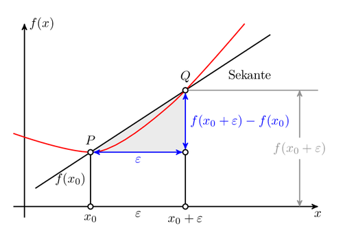
This is an illustration of linear regression.

This example was written by Henri Menke on TeXwelt.de. An animated version can be found there in addition.

Download as: [PDF] [TEX]

Do you have a question regarding this example, TikZ or LaTeX in general? Just ask in the LaTeX Forum.
Oder frag auf Deutsch auf TeXwelt.de. En français: TeXnique.fr.

% Linear regression
% Author: Henri Menke
\documentclass[tikz,border=10pt]{standalone}
\usetikzlibrary{arrows,intersections}
\begin{document}
\begin{tikzpicture}[
    thick,
    >=stealth',
    dot/.style = {
      draw,
      fill = white,
      circle,
      inner sep = 0pt,
      minimum size = 4pt
    }
  ]
  \coordinate (O) at (0,0);
  \draw[->] (-0.3,0) -- (8,0) coordinate[label = {below:$x$}] (xmax);
  \draw[->] (0,-0.3) -- (0,5) coordinate[label = {right:$f(x)$}] (ymax);
  \path[name path=x] (0.3,0.5) -- (6.7,4.7);
  \path[name path=y] plot[smooth] coordinates {(-0.3,2) (2,1.5) (4,2.8) (6,5)};
  \scope[name intersections = {of = x and y, name = i}]
    \fill[gray!20] (i-1) -- (i-2 |- i-1) -- (i-2) -- cycle;
    \draw      (0.3,0.5) -- (6.7,4.7) node[pos=0.8, below right] {Sekante};
    \draw[red] plot[smooth] coordinates {(-0.3,2) (2,1.5) (4,2.8) (6,5)};
    \draw (i-1) node[dot, label = {above:$P$}] (i-1) {} -- node[left]
      {$f(x_0)$} (i-1 |- O) node[dot, label = {below:$x_0$}] {};
    \path (i-2) node[dot, label = {above:$Q$}] (i-2) {} -- (i-2 |- i-1)
      node[dot] (i-12) {};
    \draw           (i-12) -- (i-12 |- O) node[dot,
                              label = {below:$x_0 + \varepsilon$}] {};
    \draw[blue, <->] (i-2) -- node[right] {$f(x_0 + \varepsilon) - f(x_0)$}
                              (i-12);
    \draw[blue, <->] (i-1) -- node[below] {$\varepsilon$} (i-12);
    \path       (i-1 |- O) -- node[below] {$\varepsilon$} (i-2 |- O);
    \draw[gray]      (i-2) -- (i-2 -| xmax);
    \draw[gray, <->] ([xshift = -0.5cm]i-2 -| xmax) -- node[fill = white]
      {$f(x_0 + \varepsilon)$}  ([xshift = -0.5cm]xmax);
  \endscope
\end{tikzpicture}
\end{document}