


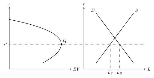
An illustration inspired by a figure in Stiglitz, J.E. and Greenwald, B. (2003). Towards a New Paradigm in Monetary Economics.
Edit and compile if you like:
% Author: Rasmus Pank Roulund
\documentclass{minimal}
\usepackage{tikz}

\usetikzlibrary{arrows,calc}
\tikzset{
%Define standard arrow tip
>=stealth',
%Define style for different line styles
help lines/.style={dashed, thick},
axis/.style={<->},
important line/.style={thick},
connection/.style={thick, dotted},
}
\begin{document}
  \begin{tikzpicture}[scale=1]
    % Axis
    \coordinate (y) at (0,5);
    \coordinate (x) at (5,0);
    \draw[<->] (y) node[above] {$r$} -- (0,0) --  (x) node[right]
    {$\mathit{EV}$};
    % A grid can be useful when defining coordinates
    % \draw[step=1mm, gray, thin] (0,0) grid (5,5);
    % \draw[step=5mm, black] (0,0) grid (5,5);

    % Let us define some coordinates
    \path
    coordinate (start) at (0,4)
    coordinate (c1) at +(5,3)
    coordinate (c2) at +(5,1.75)
    coordinate (slut) at (2.7,.5)
    coordinate (top) at (4.2,2);

    \draw[important line] (start) .. controls (c1) and (c2) .. (slut);
    % Help coordinates for drawing the curve
    % \filldraw [black]
    % (start) circle (2pt)
    % (c1) circle (2pt)
    % (c2) circle (2pt)
    % (slut) circle (2pt)
    \filldraw [black]
     (top) circle (2pt) node[above right, black] {$Q$};

     % We start the second graph
     \begin{scope}[xshift=6cm]
       % Axis
      \coordinate (y2) at (0,5);
      \coordinate (x2) at (5,0);
      \draw[axis] (y2) node[above] {$r$} -- (0,0) --  (x2) node[right] {$L$};
      % Define some coodinates
     \path
     let
     \p1=(top)
     in
     coordinate (sstart) at (1,.5)
     coordinate (sslut) at (4, 4.5)
     coordinate (dstart) at (4,.5)
     coordinate (dslut) at (1,4.5)
% Intersection 1
     coordinate (int) at  (intersection cs:
       first line={(sstart)--(sslut)},
       second line={(dstart)--(dslut)})
% Intersection 2
    coordinate (int2) at  (intersection cs:
       first line={(top)--($(10,\y1)$)},
       second line={(dstart)--(dslut)})
% Intersection 3
    coordinate (int3) at  (intersection cs:
       first line={(top)--($(10,\y1)$)},
       second line={(sstart)--(sslut)});
% Draw the lines
     \draw[important line] (sstart) -- (sslut) node[above right] {$S$}
       (dstart) -- (dslut)  node[above left] {$D$};
     \draw[connection] let \p1=(int2), \p2=(int3) in
     (int2)--(\x1,0) node[below] {$\mathit{L_D}$}
     (int3)--(\x2,0) node[below] {$\mathit{L_S}$};
      \end{scope}
%Finally, connect the two graphs
     \draw[connection] let \p1=(top), \p2=(x2) in (0,\y1) node[left]
     {$r^*$} -- (\x2, \y1);
    \end{tikzpicture}
  \end{document}
Click to download: credit-rationing.tex • credit-rationing.pdf
Open in Overleaf: credit-rationing.tex