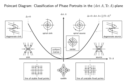
The solutions of a system of linear differential equations can be classified according to the trace and the determinant of the coefficient matrix. This diagram show schematically the different types of solutions.
Originally published on TeX.SX, tex.stackexchange.com/a/347401, 6 Jan 2017 Based on a manual drawing by Douglas R. Hundley, http://people.whitman.edu/~hundledr/courses/M244/Poincare.pdf
You may use the code without any restrictions; no rights reserved.

Edit and compile if you like:
% Poincaré Diagram: Classification of Phase Portraits in the (det A,Tr A)-plane
% Author: Gernot Salzer, 22 Jan 2017
\documentclass[tikz,border=10pt]{standalone}
\usetikzlibrary{decorations.markings}

\tikzset
 {every pin/.style = {pin edge = {<-}},    % pins are arrows from label to point
  > = stealth,                            % arrow tips look like stealth bombers
  flow/.style =    % everything marked as "flow" will be decorated with an arrow
   {decoration = {markings, mark=at position #1 with {\arrow{>}}},
    postaction = {decorate}
   },
  flow/.default = 0.5,          % default position of the arrow is in the middle
  main/.style = {line width=1pt}                    % thick lines for main graph
 }

% \newtemplate[Scaling, default 0.18]{\NameOfTemplate}{Caption}{Code}
%
% Typesets Code and stores it in the box \NameOfTemplate.
% This way we avoid nested tikzpictures when inserting the templates into the
% main picture, since nesting is not guaranteed to work.
\newcommand\newtemplate[4][0.18]%
 {\newsavebox#2%
  \savebox#2%
   {\begin{tabular}{@{}c@{}}
      \begin{tikzpicture}[scale=#1]
      #4
      \end{tikzpicture}\\[-1ex]
      \templatecaption{#3}\\[-1ex]
    \end{tabular}%
   }%
 }
\newcommand\template[1]{\usebox{#1}}             % use the Code stored in box #1
\newcommand\templatecaption[1]{{\sffamily\scriptsize#1}}       % typeset caption
\newcommand\Tr{\mathop{\mathrm{Tr}}}

\newtemplate\sink{sink}%
 {\foreach \sx in {+,-}                   % for right/left half do:
   {\draw[flow] (\sx4,0) -- (0,0);        %   draw half of horizontal axis
    \draw[flow] (0,\sx4) -- (0,0);        %   draw half of vertical axis
    \foreach \sy in {+,-}                 %   for upper/lower quadrant do:
      \foreach \a/\b in {2/1,3/0.44}      %     draw two half-parabolas
        \draw[flow,domain=\sx\a:0] plot (\x, {\sy\b*\x*\x});
   }
 }

\newtemplate\source{source}%
 {\foreach \sx in {+,-}                   % for right/left half do:
   {\draw[flow] (0,0) -- (\sx4,0);        %   draw half of horizontal axis
    \draw[flow] (0,0) -- (0,\sx4);        %   draw half of vertical axis
    \foreach \sy in {+,-}                 %   for upper/lower quadrant do:
      \foreach \a/\b in {2/1,3/0.44}      %     draw two half-parabolas
        \draw[flow,domain=0:\sx\a] plot (\x, {\sy\b*\x*\x});
   }
 }

\newtemplate\stablefp{line of stable fixed points}%
 {\draw (-4,0) -- (4,0);                  % draw horizontal axis
  \foreach \sy in {+,-}                   % for upper/lower half do:
   {\draw[flow] (0,\sy4) -- (0,0);        %   draw half of vertical axis
    \foreach \x in {-3,-2,-1,1,2,3}       %   draw six vertical half-lines
      \draw[flow] (\x,\sy3) -- (\x,0);
   }
 }

\newtemplate\unstablefp{line of unstable fixed points}%
 {\draw (-4,0) -- (4,0);                  % draw horizontal axis
  \foreach \sy in {+,-}                   % for upper/lower half do:
   {\draw[flow] (0,0) -- (0,\sy4);        %   draw half of vertical axis
    \foreach \x in {-3,-2,-1,1,2,3}       %   draw six vertical half-lines
      \draw[flow] (\x,0) -- (\x,\sy3);
   }
 }

\newtemplate\spiralsink{spiral sink}%
 {\draw (-4,0) -- (4,0);                  % draw horizontal axis
  \draw (0,-4) -- (0,4);                  % draw vertical axis
  \draw [samples=100,smooth,domain=27:7]  % draw spiral
       plot ({\x r}:{0.005*\x*\x});       % Using "flow" here gives "Dimension
  \def\x{26}                              %        too large", so we draw a tiny
  \draw[->] ({\x r}:{0.005*\x*\x}) -- +(0.01,-0.01);%     tangent for the arrow.
 }

\newtemplate\spiralsource{spiral source}%
 {\draw (-4,0) -- (4,0);                  % draw horizontal axis
  \draw (0,-4) -- (0,4);                  % draw vertical axis
  \draw [samples=100,smooth,domain=10:28] % draw spiral
       plot ({-\x r}:{0.005*\x*\x});      % Using "flow" here gives "Dimension
  \def\x{27.5}                            %        too large", so we draw a tiny
  \draw[<-] ({-\x r}:{0.005*\x*\x}) -- +(0.01,-0.008);%   tangent for the arrow.
 }

\newtemplate[0.15]\centre{center}% British spelling since \center is in use
 {\draw (-4,0) -- (4,0);                  % draw horizontal axis
  \draw (0,-4) -- (0,4);                  % draw vertical axis
  \foreach \r in {1,2,3}                  % draw three circles
    \draw[flow=0.63] (\r,0) arc (0:-360:\r cm);
 }

\newtemplate\saddle{saddle}%
 {\foreach \sx in {+,-}                   % for right/left half do:
   {\draw[flow] (\sx4,0) -- (0,0);        %   draw half of horizontal axis
    \draw[flow] (0,0) -- (0,\sx4);        %   draw half of vertical axis
    \foreach \sy in {+,-}                 %   for upper/lower quadrant do:
      \foreach \a/\b/\c/\d in {2.8/0.3/0.7/0.6, 3.9/0.4/1.3/1.1}
        \draw[flow] (\sx\a,\sy\b)         %     draw two bent lines
          .. controls (\sx\c,\sy\d) and (\sx\d,\sy\c)
          .. (\sx\b,\sy\a);
   }
 }

\newtemplate\degensink{degenerate sink}%
 {\draw (0,-4) -- (0,4);                  % draw vertical axis
  \foreach \s in {+,-}                    % for upper/lower half do:
   {\draw[flow] (\s4,0) -- (0,0);         %   draw half of horizontal axis
    \foreach \a/\b/\c/\d in {3.5/4/1.5/1, 2.5/2/1/0.8}
      \draw[flow] (\s-3.5,\s\a)           %   draw two bent lines
        .. controls (\s\b,\s\c) and (\s\b,\s\d)
        .. (0,0);
   }
 }

\newtemplate\degensource{degenerate source}%
 {\draw (0,-4) -- (0,4);                  % draw vertical axis
  \foreach \s in {+,-}                    % for upper/lower half do:
   {\draw[flow] (0,0) -- (\s4,0);         %   draw half of horizontal axis
    \foreach \a/\b/\c/\d in {3.5/4/1.5/1, 2.5/2/1/0.8}
      \draw[flow] (0,0)                   %   draw two bent lines
        .. controls (\s\b,\s\d) and (\s\b,\s\c)
        .. (\s-3.5,\s\a);
   }
 }

\begin{document}
\begin{tikzpicture}[line cap=round,line join=round]
  % MAIN DIAGRAM
  \draw [main,->] (0,-0.3) -- (0,4.7)                            % vertical axis
    node [label={[above]$\scriptstyle\det A$}] {}
    node [label={[above,yshift=0.8cm]%
      {\sffamily\large Poincar\'e Diagram: Classification of Phase
      Portraits in the $(\det A,\Tr A)$-plane}}] {};
  \draw [main,->] (-5,0) -- (5,0)                              % horizontal axis
    node [label={[right,yshift=-0.5ex]$\scriptstyle\Tr A$}] {};
  \draw [main, domain=-4:4] plot (\x, {0.25*\x*\x});                % main graph
  \node at (-4,4) [pin={[above]$\scriptstyle\Delta=0$}] {};
  \node at ( 4,4) [pin={[above,align=left]%
    {$\scriptstyle\Delta=0:\;\det A=\frac{1}{4}(\Tr A)^2$}}] {};
  % TEMPLATES describing areas
  \node at ( 0  ,-1.4) {\template\saddle};
  \node at (-4  , 1  ) {\template\sink};
  \node at ( 4  , 1  ) {\template\source};
  \node at (-1.8, 3.7) {\template\spiralsink};
  \node at ( 1.8, 3.7) {\template\spiralsource};
  % TEMPLATES labeling lines and points
  \node at ( 0  , 1.2) [pin={[draw,right,xshift=0.3cm]%
    \template\centre}] {};
  \node at (-3  , 0  ) [pin={[draw,below,yshift=-1cm]%
    \template\stablefp}] {};
  \node at ( 3  , 0  ) [pin={[draw,below,yshift=-1cm]%
    \template\unstablefp}] {};
  \node at (-3.5,{0.25*3.5*3.5}) [pin={[draw,left,xshift=-1.15cm,yshift=-0.3cm]%
    \template\degensink}] {};
  \node at ( 3.5,{0.25*3.5*3.5}) [pin={[draw,right,xshift=0.9cm,yshift=-0.3cm]%
    \template\degensource}] {};
  \node at ( 0  , 0  ) [pin={[draw,above left,align=center,xshift=-0.3cm]%
    \templatecaption{uniform}\\[-1ex]\templatecaption{motion}}] {};
\end{tikzpicture}
\end{document}
Click to download: poincare.tex • poincare.pdf
Open in Overleaf: poincare.tex


