Example: Spherical polar pots with 3dplot

Published 2009-12-04 | Author: Jeff Hein

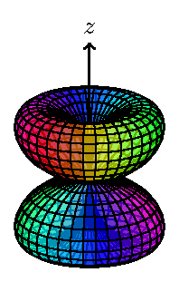
The 3dplot package has been extended to handle the plotting of user-specified functions in spherical polar coordinates. In this example, a spherical harmonic is rendered, where the fill hue represents the complex phase angle. More info about spherical harmonics can be found at http://en.wikipedia.org/wiki/Spherical_harmonics.

The 3dplot.sty package can be found at http://www.heinjd.com/dev/latex/3dplot/3dplot.sty.

Documentation for the 3dplot.sty package can be found at http://www.heinjd.com/dev/latex/3dplot/3dplot_documentation.pdf.

Download as: [PDF] [TEX] [ZIP]

Do you have a question regarding this example, TikZ or LaTeX in general? Just ask in the LaTeX Forum.
Oder frag auf Deutsch auf TeXwelt.de. En français: TeXnique.fr.

%harmonics.tex: produces spherical harmonic plots using the 3dplot package
% Author: Jeff Hein
\documentclass{minimal}
\usepackage{tikz}           %for TikZ graphics
\usepackage{3dplot} %for 3dplot functionality

\usepackage[active,tightpage]{preview}      %generates a tightly fitting border around the work
\PreviewEnvironment{tikzpicture}
\setlength\PreviewBorder{2mm}

\begin{document}
\tdplotsetmaincoords{70}{135}
\begin{tikzpicture}[line join=bevel,tdplot_main_coords, fill opacity=.7]
\tdplotsphericalsurfaceplot[parametricfill]{72}{36}%
{sqrt(15/2)*sin(\tdplottheta)*cos(\tdplottheta)}{black}{\tdplotphi}%
    {\draw[color=black,thick,->] (0,0,0) -- (2,0,0) node[anchor=north east]{$x$};}%
    {\draw[color=black,thick,->] (0,0,0) -- (0,2,0) node[anchor=north west]{$y$};}%
    {\draw[color=black,thick,->] (0,0,0) -- (0,0,2) node[anchor=south]{$z$};}%
\end{tikzpicture}

%Here's some more examples.
%L = 0
%\begin{tikzpicture}[scale=2,line join=bevel,tdplot_main_coords, fill opacity=.7]
%\tdplotsphericalsurfaceplot[parametricfill]{72}{36}%
%{1}{black}{0}%
%   {\draw[color=black,thick,->] (0,0,0) -- (2,0,0) node[anchor=north east]{$x$};}%
%   {\draw[color=black,thick,->] (0,0,0) -- (0,2,0) node[anchor=north west]{$y$};}%
%   {\draw[color=black,thick,->] (0,0,0) -- (0,0,2) node[anchor=south]{$z$};}%
%\end{tikzpicture}
%
%L = 1, M_L = -1
%\begin{tikzpicture}[scale=2,line join=bevel,tdplot_main_coords, fill opacity=.7]
%\tdplotsphericalsurfaceplot[parametricfill]{72}{36}%
%{sqrt(3/2)*sin(\tdplottheta)}{black}{-\tdplotphi}%
%   {\draw[color=black,thick,->] (0,0,0) -- (2,0,0) node[anchor=north east]{$x$};}%
%   {\draw[color=black,thick,->] (0,0,0) -- (0,2,0) node[anchor=north west]{$y$};}%
%   {\draw[color=black,thick,->] (0,0,0) -- (0,0,2) node[anchor=south]{$z$};}%
%\end{tikzpicture}
%
%L = 1, M_L = 0
%\begin{tikzpicture}[scale=2,line join=bevel,tdplot_main_coords, fill opacity=.7]
%\tdplotsphericalsurfaceplot[parametricfill]{72}{36}%
%{sqrt(3)*cos(\tdplottheta)}{black}{0}%
%   {\draw[color=black,thick,->] (0,0,0) -- (2,0,0) node[anchor=north east]{$x$};}%
%   {\draw[color=black,thick,->] (0,0,0) -- (0,2,0) node[anchor=north west]{$y$};}%
%   {\draw[color=black,thick,->] (0,0,0) -- (0,0,2) node[anchor=south]{$z$};}%
%\end{tikzpicture}
%
%L = 1, M_L = +1
%\begin{tikzpicture}[scale=2,line join=bevel,tdplot_main_coords, fill opacity=.7]
%\tdplotsphericalsurfaceplot[parametricfill]{72}{36}%
%{sqrt(3/2)*sin(\tdplottheta)}{black}{\tdplotphi}%
%   {\draw[color=black,thick,->] (0,0,0) -- (2,0,0) node[anchor=north east]{$x$};}%
%   {\draw[color=black,thick,->] (0,0,0) -- (0,2,0) node[anchor=north west]{$y$};}%
%   {\draw[color=black,thick,->] (0,0,0) -- (0,0,2) node[anchor=south]{$z$};}%
%\end{tikzpicture}
%
%L = 2, M_L = -2
%\begin{tikzpicture}[line join=bevel,tdplot_main_coords, fill opacity=.7]
%\tdplotsphericalsurfaceplot[parametricfill]{72}{36}%
%{sqrt(15/2)/2*sin(\tdplottheta)^2}{black}{-2*\tdplotphi}%
%   {\draw[color=black,thick,->] (0,0,0) -- (2,0,0) node[anchor=north east]{$x$};}%
%   {\draw[color=black,thick,->] (0,0,0) -- (0,2,0) node[anchor=north west]{$y$};}%
%   {\draw[color=black,thick,->] (0,0,0) -- (0,0,2) node[anchor=south]{$z$};}%
%\end{tikzpicture}
%
%L = 2, M_L = -1
%\begin{tikzpicture}[line join=bevel,tdplot_main_coords, fill opacity=.7]
%\tdplotsphericalsurfaceplot[parametricfill]{72}{36}%
%{sqrt(15/2)*sin(\tdplottheta)*cos(\tdplottheta)}{black}{-\tdplotphi}%
%   {\draw[color=black,thick,->] (0,0,0) -- (2,0,0) node[anchor=north east]{$x$};}%
%   {\draw[color=black,thick,->] (0,0,0) -- (0,2,0) node[anchor=north west]{$y$};}%
%   {\draw[color=black,thick,->] (0,0,0) -- (0,0,2) node[anchor=south]{$z$};}%
%\end{tikzpicture}
%
%L = 2, M_L = 0
%\begin{tikzpicture}[line join=bevel,tdplot_main_coords, fill opacity=.7]
%\tdplotsphericalsurfaceplot[parametricfill]{72}{36}%
%{sqrt(5)/2*(3*cos(\tdplottheta)^2 - 1 )}{black}{-\tdplotphi}%
%   {\draw[color=black,thick,->] (0,0,0) -- (2,0,0) node[anchor=north east]{$x$};}%
%   {\draw[color=black,thick,->] (0,0,0) -- (0,2,0) node[anchor=north west]{$y$};}%
%   {\draw[color=black,thick,->] (0,0,0) -- (0,0,2) node[anchor=south]{$z$};}%
%\end{tikzpicture}
%
%L = 2, M_L = 1
%\begin{tikzpicture}[line join=bevel,tdplot_main_coords, fill opacity=.7]
%\tdplotsphericalsurfaceplot[parametricfill]{72}{36}%
%{sqrt(15/2)*sin(\tdplottheta)*cos(\tdplottheta)}{black}{\tdplotphi}%
%   {\draw[color=black,thick,->] (0,0,0) -- (2,0,0) node[anchor=north east]{$x$};}%
%   {\draw[color=black,thick,->] (0,0,0) -- (0,2,0) node[anchor=north west]{$y$};}%
%   {\draw[color=black,thick,->] (0,0,0) -- (0,0,2) node[anchor=south]{$z$};}%
%\end{tikzpicture}
%
%L = 2, M_L = +2
%\begin{tikzpicture}[line join=bevel,tdplot_main_coords, fill opacity=.7]
%\tdplotsphericalsurfaceplot[parametricfill]{72}{36}%
%{sqrt(15/2)/2*sin(\tdplottheta)^2}{black}{2*\tdplotphi}%
%   {\draw[color=black,thick,->] (0,0,0) -- (2,0,0) node[anchor=north east]{$x$};}%
%   {\draw[color=black,thick,->] (0,0,0) -- (0,2,0) node[anchor=north west]{$y$};}%
%   {\draw[color=black,thick,->] (0,0,0) -- (0,0,2) node[anchor=south]{$z$};}%
%\end{tikzpicture}

%L = 3, M_L = 0
%\begin{tikzpicture}[line join=bevel,tdplot_main_coords, fill opacity=.7]
%\tdplotsphericalsurfaceplot[parametricfill]{72}{36}%
%{sqrt(7)/2*(5*cos(\tdplottheta)^3 - 3*cos(\tdplottheta))}{black}{0}%
%   {\draw[color=black,thick,->] (0,0,0) -- (2,0,0) node[anchor=north east]{$x$};}%
%   {\draw[color=black,thick,->] (0,0,0) -- (0,2,0) node[anchor=north west]{$y$};}%
%   {\draw[color=black,thick,->] (0,0,0) -- (0,0,2) node[anchor=south]{$z$};}%
%\end{tikzpicture}


\end{document}

Comments

#1 Jeff Hein, December 4, 2009 at 8:15 p.m.

Just an extra note. Since this project is a work in progress, you can expect there to be changes to the 3dplot.sty file. I'll be noting changes at http://heinjd.wordpress.com/category/3dplot/ if you are interested.
#2 Kjell Magne Fauske, December 4, 2009 at 8:34 p.m.

Thanks for the link Jeff. You should upload it to CTAN as well.
#3 Rafa Gallego, December 4, 2009 at 8:41 p.m.

Congratulations!!! This is certainly a very nice and promising package. I encourage you to keep on developing it and I also think that you should upload it to CTAN. Good job.
#4 Dave, December 7, 2009 at 12:06 a.m.

Nice, how do I get the plot to appear after text. When I include this code, the text doesn't show up.

#5 Kjell Magne Fauske, December 7, 2009 at 8:59 a.m.

@Dave. Remove the following code lines:

\usepackage[active,tightpage]{preview}
\PreviewEnvironment{tikzpicture}
\setlength\PreviewBorder{2mm}

#6 Jeff Hein, January 21, 2010 at 1:32 a.m.

I have uploaded a renamed version of this package to CTAN. you can find "tikz-3dplot" at [http://www.ctan.org/tex-archive/graphics/pgf/contrib/tikz-3dplot/] where it will be maintained from now on.