


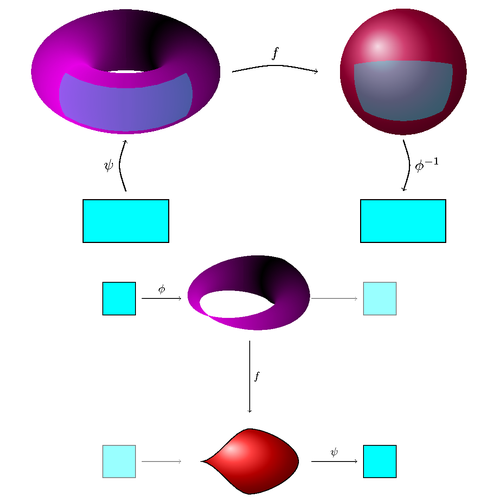
Illustrations from the talk "Comparative Smootheology: Workshop on Smooth Structures in Ottawa". More illustrations from the talk are available on the author's web site.
Edit and compile if you like:
% Smooth map of manifolds and smooth spaces
% Author: Andrew Stacey
% Source: http://www.math.ntnu.no/~stacey/Seminars/ottawa.html
\documentclass{article}
\thispagestyle{empty}
%\def\pgfsysdriver{pgfsys-tex4ht.def}
\usepackage{tikz}
\usepackage[active,tightpage]{preview}
\PreviewEnvironment{tikzpicture}
\setlength\PreviewBorder{5pt}%


\begin{document}

\begin{tikzpicture}
    % \x runs over the angles at which to draw the circles defining the
    % torus
    \foreach \x in {90,89,...,-90} { % change 89 to 80 or 45 for speed
    % \elrad is the x-radius of the ellipse (technically, a circle seen
    % from side on at angle \x).  The 'max' is because at small angles
    % then the real ellipse is too thin and the torus doesn't ``fill
    % out'' nicely.
    \pgfmathsetmacro\elrad{20*max(cos(\x),.1)}
    % We draw the torus from the back to the front to get the right
    % layering effect.  To tint it, we define colours according to the
    % angle, but need different colours for the left and right pieces.
    % It'd be nice if the xcolor colour specification could take something
    % computed by pdfmath, such as {red!\tint} but it doesn't appear to
    % work, so we define the colours explicitly.
    \pgfmathsetmacro\ltint{.9*abs(\x-45)/180}
    \pgfmathsetmacro\rtint{.9*(1-abs(\x+45)/180)}
    \definecolor{currentcolor}{rgb}{\ltint, 0, \ltint}
    % This draws the right-hand circle.
    \draw[color=currentcolor,fill=currentcolor]
        (xyz polar cs:angle=\x,y radius=.75,x radius=1.5)
        ellipse (\elrad pt and 20pt);
    % This sets the colour correctly for the left-hand circle ...
    \definecolor{currentcolor}{rgb}{\rtint, 0, \rtint}
    % ... and draws it
    \draw[color=currentcolor,fill=currentcolor]
        (xyz polar cs:angle=180-\x,radius=.75,x radius=1.5)
        ellipse (\elrad pt and 20pt);
    % End of foreach statement
    }
    % Spheres are *much* easier!
    \shadedraw[shading=ball,ball color=purple, white] (6.5,0) circle (1.5);
    % As are the subsets of Euclidean space
    \draw[fill=cyan] (-1,-4) rectangle (1,-3);
    \draw[fill=cyan] (5.5,-4) rectangle (7.5,-3);
    % The next three draw the maps, slightly curved for aesthetics.
    \draw[->] (0,-2.8) .. controls (-.2,-2.2) .. (0,-1.6)
        node[pos=0.5, auto=left] {\(\psi\)};
    \draw[->] (6.5,-1.6) .. controls (6.7,-2.2) .. (6.5,-2.8)
        node[pos=0.5, auto=left] {\(\phi^{-1}\)};
    \draw[->] (2.5,0) .. controls (3.5,.2) .. (4.5,0)
        node[pos=0.5, auto=left] {\(f\)};
    % Now we want to draw the codomains of the charts.  Sticking cosines
    % and sines directly into the coordinates doesn't seem to work so
    % we define macros to hold the sines and cosines of the angles.
    % \elrad is the angle on the torus at which to start.
    \pgfmathsetmacro\elrad{cos(-135)}
    % the circle drawn at the specific angle on the torus looks like an
    % ellipse, \xrad and \yrad compute its major and minor semi-axes.
    \pgfmathsetmacro\xrad{1.5cm-20pt*\elrad}
    \pgfmathsetmacro\yrad{.75cm-20pt*sin(-135)}
    % This draws the codomain of the chart on the torus.
    \path[fill=cyan, fill opacity=.35]
        (xyz polar cs:angle=-135,radius=.75,x radius=1.5)
        ++(20pt*\elrad,0) arc (0:45:20*\elrad pt and 20pt)
        arc (-135:-45:\xrad pt and \yrad pt)
        arc (45:-45:-20*\elrad pt and 20pt)
        arc (-45:-135:\xrad pt and \yrad pt)
        arc (-45:0:20*\elrad pt and 20pt);
    % Now we do the same for the sphere.
    % We do this by drawing some great circles (aka ellipses) on the
    % sphere and then ``clipping'' an overlaid (and slightly trans:parent)
    % sphere by those great circles.  Each great circle actually specifies
    % one side of the ``clip'' so to make sure that the clip is big enough
    % the arcs are completed by big rectangles (otherwise the clipping
    % would join the end points directly).
    \pgfmathsetmacro\tell{-sin(10)}
    \pgfmathsetmacro\bell{sin(50)}
    \pgfmathsetmacro\rell{1.5 * sin(50)}
    \begin{scope}
        \clip (6.5,0) +(-1.5,0) arc (-180:0:1.5 and 1.5*\tell)
            -- ++(0,-1.5) -- ++(-3,0) -- ++(0,1.5);
        \clip (6.5,0) +(-1.5,0) arc (-180:0:1.5 and 1.5*\bell)
            -- ++(0,1.5) -- ++(-3,0) -- ++(0,-1.5);
        \clip (6.5,0) +(0,1.5)  arc (90:-90:\rell cm and 1.5 cm)
            -- ++(-1.5,0) -- ++(0,3) -- ++(1.5,0);
        \clip (6.5,0) +(0,1.5)  arc (90:-90:-\rell cm and 1.5 cm)
            -- ++(1.5,0) -- ++(0,3) -- ++(-1.5,0);
        \fill[cyan, fill opacity=0.35] (6.5,0) circle (1.5);
    \end{scope}
\end{tikzpicture}

\begin{tikzpicture}
    \draw[fill=cyan] (0,0) rectangle (1,-1);
    \draw[gray,fill=cyan!40!white] (8,0) rectangle (9,-1);
    \draw[gray,fill=cyan!40!white] (0,-5) rectangle (1,-6);
    \draw[fill=cyan] (8,-5) rectangle (9,-6);
    \foreach \x in {90,89,...,-90} { % change 89 to 80 for speed
        % \elrad is the x-radius of the ellipse (technically, a circle seen
        % from side on at angle \x).  The 'max' is because at small angles
        % then the real ellipse is too thin and the torus doesn't ``fill
        % out'' nicely.
        \pgfmathsetmacro\elrad{20*max(cos(\x),.1)}
        \pgfmathsetmacro\lscale{1-abs(\x-45)/180}
        \pgfmathsetmacro\rscale{abs(\x+45)/180}
        % We draw the torus from the back to the front to get the right
        % layering effect.  To tint it, we define colours according to the
        % angle, but need different colours for the left and right pieces.
        % It'd be nice if the xcolor colour specification could take something
        % computed by pdfmath, such as {red!\tint} but it doesn't appear to
        % work, so we define the colours explicitly.
        \pgfmathsetmacro\ltint{.9*abs(\x-45)/180}
        \pgfmathsetmacro\rtint{.9*(1-abs(\x+45)/180)}
        \definecolor{currentcolor}{rgb}{\ltint, 0, \ltint}
        % This draws the right-hand circle.
        \draw[color=currentcolor,fill=currentcolor] (4.3cm,-.5cm)
            +(xyz polar cs:angle=\x,y radius=.75,x radius=1.5)
            ellipse (\elrad*\lscale pt and 20*\lscale pt);
        % This sets the colour correctly for the left-hand circle ...
        \definecolor{currentcolor}{rgb}{\rtint, 0, \rtint}
        % ... and draws it
        \draw[color=currentcolor,fill=currentcolor] (4.3cm,-.5cm)
            +(xyz polar cs:angle=180-\x,radius=.75,x radius=1.5)
            ellipse (\elrad*\rscale pt and 20*\rscale pt);
    % End of foreach statement
    }
    \shadedraw[shading=ball,ball color=red] (3,-5.5)
        .. controls (3.5,-5.5) and (4,-4.5) .. (4.5,-4.5)
        .. controls (5,-4.5) and (6,-5) .. (6,-5.5)
        .. controls (6,-6) and (5,-6.5) .. (4.5,-6.5)
        .. controls (4,-6.5) and (3.5, -5.5) .. (3,-5.5);
    \draw[->] (1.2,-0.5) -- node[auto=left] {\(\phi\)} (2.4,-0.5);
    \draw[->, color=gray] (1.2,-5.5) -- (2.4,-5.5);
    \draw[->, color=gray] (6.4,-0.5) -- (7.8,-0.5);
    \draw[->] (6.4,-5.5) -- node[auto=left] {\(\psi\)} (7.8,-5.5);
    \draw[->] (4.5,-1.8) -- node[auto=left] {\(f\)} (4.5,-4);
\end{tikzpicture}
\end{document}
Click to download: smooth-maps.tex • smooth-maps.pdf
Open in Overleaf: smooth-maps.tex