SWAN wave model

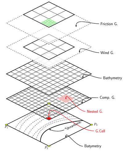
SWAN (developed by SWAN group, TU Delft, The Netherlands) is a wave spectral numerical model. For Simlating WAves Nearshore, it is necessary to define spatial grids of physical dominant factors (wind friction, dissipation) as well as define a COMPUTATIONAL grid on which the model performs its (spectral) calculations: budgeting energy spectra over each cell of the (computational) grid. Grids might have different spatial resolution and extension.

Edit and compile if you like:

1
2
3
4
5
6
7
8
9
10
11
12
13
14
15
16
17
18
19
20
21
22
23
24
25
26
27
28
29
30
31
32
33
34
35
36
37
38
39
40
41
%Author: Marco Miani
%SWAN (developed by SWAN group, TU Delft, The Netherlands) is a wave spectral numerical model.
%For Simlating WAves Nearshore, it is necessary to define spatial grids of
%physical dominant factors (wind friction, dissipation) as well as define a COMPUTATIONAL
%grid on which the model performs its (spectral) calculations: budgeting energy spectra over
%each cell of the (computational) grid. Grids might have different spatial resolution and extension.
\documentclass[12pt]{article}
\usepackage{tikz}
\usetikzlibrary{positioning}
\begin{document}
\pagestyle{empty}
\begin{tikzpicture}[scale=.9,every node/.style={minimum size=1cm},on grid]
        
    %slanting: production of a set of n 'laminae' to be piled up. N=number of grids.
    \begin{scope}[
            yshift=-83,every node/.append style={
            yslant=0.5,xslant=-1},yslant=0.5,xslant=-1
            ]
        % opacity to prevent graphical interference
        \fill[white,fill opacity=0.9] (0,0) rectangle (5,5);
        \draw[step=4mm, black] (0,0) grid (5,5); %defining grids
        \draw[step=1mm, red!50,thin] (3,1) grid (4,2);  %Nested Grid
        \draw[black,very thick] (0,0) rectangle (5,5);%marking borders
        \fill[red] (0.05,0.05) rectangle (0.35,0.35);
        %Idem as above, for the n-th grid:
    \end{scope}
        
    \begin{scope}[
        yshift=0,every node/.append style={
            yslant=0.5,xslant=-1},yslant=0.5,xslant=-1
                     ]
        \fill[white,fill opacity=.9] (0,0) rectangle (5,5);
        \draw[black,very thick] (0,0) rectangle (5,5);
        \draw[step=5mm, black] (0,0) grid (5,5);
    \end{scope}
        
    \begin{scope}[
 
 
הההההההההההההההההההההההההההההההההההההההההההההההההההההההההההההההההההההההההההההההההההההההההההההההההההההההההההההההההההההההההההההההההההההההההההההההההההההההההההההההההההההההההההההההההההההההההההההההההההההההההההההההההההההההההההההההההההההההההההההההההההההההההההההההה
XXXXXXXXXXXXXXXXXXXXXXXXXXXXXXXXXXXXXXXXXXXXXXXXXXXXXXXXXXXXXXXXXXXXXXXXXXXXXXXXXXXXXXXXXXXXXXXXXXXXXXXXXXXXXXXXXXXXXXXXXXXXXXXXXXXXXXXXXXXXXXXXXXXXXXXXXXXXXXXXXXXXXXXXXXXXXXXXXXXXXXXXXXXXXXXXXXXXXXXXXXXXXXXXXXXXXXXXXXXXXXXXXXXXXXXXXXXXXXXXXXXXXXXXXXXXXXXX