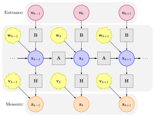
This is the system model of the (linear) Kalman filter.

Edit and compile if you like:
% Kalman filter system model
% by Burkart Lingner
% An example using TikZ/PGF 2.00
%
% Features: Decorations, Fit, Layers, Matrices, Styles
% Tags: Block diagrams, Diagrams
% Technical area: Electrical engineering

\documentclass[a4paper,10pt]{article}

\usepackage[english]{babel}
\usepackage[T1]{fontenc}
\usepackage[ansinew]{inputenc}

\usepackage{lmodern}	% font definition
\usepackage{amsmath}	% math fonts
\usepackage{amsthm}
\usepackage{amsfonts}

\usepackage{tikz}

\usepackage[active,tightpage]{preview}
\PreviewEnvironment{tikzpicture}
\setlength\PreviewBorder{5pt}%


\usetikzlibrary{decorations.pathmorphing} % noisy shapes
\usetikzlibrary{fit}					% fitting shapes to coordinates
\usetikzlibrary{backgrounds}	% drawing the background after the foreground

\begin{document}

\begin{figure}[htbp]
\centering
% The state vector is represented by a blue circle.
% "minimum size" makes sure all circles have the same size
% independently of their contents.
\tikzstyle{state}=[circle,
                                    thick,
                                    minimum size=1.2cm,
                                    draw=blue!80,
                                    fill=blue!20]

% The measurement vector is represented by an orange circle.
\tikzstyle{measurement}=[circle,
                                                thick,
                                                minimum size=1.2cm,
                                                draw=orange!80,
                                                fill=orange!25]

% The control input vector is represented by a purple circle.
\tikzstyle{input}=[circle,
                                    thick,
                                    minimum size=1.2cm,
                                    draw=purple!80,
                                    fill=purple!20]

% The input, state transition, and measurement matrices
% are represented by gray squares.
% They have a smaller minimal size for aesthetic reasons.
\tikzstyle{matrx}=[rectangle,
                                    thick,
                                    minimum size=1cm,
                                    draw=gray!80,
                                    fill=gray!20]

% The system and measurement noise are represented by yellow
% circles with a "noisy" uneven circumference.
% This requires the TikZ library "decorations.pathmorphing".
\tikzstyle{noise}=[circle,
                                    thick,
                                    minimum size=1.2cm,
                                    draw=yellow!85!black,
                                    fill=yellow!40,
                                    decorate,
                                    decoration={random steps,
                                                            segment length=2pt,
                                                            amplitude=2pt}]

% Everything is drawn on underlying gray rectangles with
% rounded corners.
\tikzstyle{background}=[rectangle,
                                                fill=gray!10,
                                                inner sep=0.2cm,
                                                rounded corners=5mm]

\begin{tikzpicture}[>=latex,text height=1.5ex,text depth=0.25ex]
    % "text height" and "text depth" are required to vertically
    % align the labels with and without indices.

  % The various elements are conveniently placed using a matrix:
  \matrix[row sep=0.5cm,column sep=0.5cm] {
    % First line: Control input
    &
        \node (u_k-1) [input]{$\mathbf{u}_{k-1}$}; &
        &
        \node (u_k)   [input]{$\mathbf{u}_k$};     &
        &
        \node (u_k+1) [input]{$\mathbf{u}_{k+1}$}; &
        \\
        % Second line: System noise & input matrix
        \node (w_k-1) [noise] {$\mathbf{w}_{k-1}$}; &
        \node (B_k-1) [matrx] {$\mathbf{B}$};       &
        \node (w_k)   [noise] {$\mathbf{w}_k$};     &
        \node (B_k)   [matrx] {$\mathbf{B}$};       &
        \node (w_k+1) [noise] {$\mathbf{w}_{k+1}$}; &
        \node (B_k+1) [matrx] {$\mathbf{B}$};       &
        \\
        % Third line: State & state transition matrix
        \node (A_k-2)         {$\cdots$};           &
        \node (x_k-1) [state] {$\mathbf{x}_{k-1}$}; &
        \node (A_k-1) [matrx] {$\mathbf{A}$};       &
        \node (x_k)   [state] {$\mathbf{x}_k$};     &
        \node (A_k)   [matrx] {$\mathbf{A}$};       &
        \node (x_k+1) [state] {$\mathbf{x}_{k+1}$}; &
        \node (A_k+1)         {$\cdots$};           \\
        % Fourth line: Measurement noise & measurement matrix
        \node (v_k-1) [noise] {$\mathbf{v}_{k-1}$}; &
        \node (H_k-1) [matrx] {$\mathbf{H}$};       &
        \node (v_k)   [noise] {$\mathbf{v}_k$};     &
        \node (H_k)   [matrx] {$\mathbf{H}$};       &
        \node (v_k+1) [noise] {$\mathbf{v}_{k+1}$}; &
        \node (H_k+1) [matrx] {$\mathbf{H}$};       &
        \\
        % Fifth line: Measurement
        &
        \node (z_k-1) [measurement] {$\mathbf{z}_{k-1}$}; &
        &
        \node (z_k)   [measurement] {$\mathbf{z}_k$};     &
        &
        \node (z_k+1) [measurement] {$\mathbf{z}_{k+1}$}; &
        \\
    };

    % The diagram elements are now connected through arrows:
    \path[->]
        (A_k-2) edge[thick] (x_k-1)	% The main path between the
        (x_k-1) edge[thick] (A_k-1)	% states via the state
        (A_k-1) edge[thick] (x_k)		% transition matrices is
        (x_k)   edge[thick] (A_k)		% accentuated.
        (A_k)   edge[thick] (x_k+1)	% x -> A -> x -> A -> ...
        (x_k+1) edge[thick] (A_k+1)

        (x_k-1) edge (H_k-1)				% Output path x -> H -> z
        (H_k-1) edge (z_k-1)
        (x_k)   edge (H_k)
        (H_k)   edge (z_k)
        (x_k+1) edge (H_k+1)
        (H_k+1) edge (z_k+1)

        (v_k-1) edge (z_k-1)				% Output noise v -> z
        (v_k)   edge (z_k)
        (v_k+1) edge (z_k+1)

        (w_k-1) edge (x_k-1)				% System noise w -> x
        (w_k)   edge (x_k)
        (w_k+1) edge (x_k+1)

        (u_k-1) edge (B_k-1)				% Input path u -> B -> x
        (B_k-1) edge (x_k-1)
        (u_k)   edge (B_k)
        (B_k)   edge (x_k)
        (u_k+1) edge (B_k+1)
        (B_k+1) edge (x_k+1)
        ;

    % Now that the diagram has been drawn, background rectangles
    % can be fitted to its elements. This requires the TikZ
    % libraries "fit" and "background".
    % Control input and measurement are labeled. These labels have
    % not been translated to English as "Measurement" instead of
    % "Messung" would not look good due to it being too long a word.
    \begin{pgfonlayer}{background}
        \node [background,
                    fit=(u_k-1) (u_k+1),
                    label=left:Entrance:] {};
        \node [background,
                    fit=(w_k-1) (v_k-1) (A_k+1)] {};
        \node [background,
                    fit=(z_k-1) (z_k+1),
                    label=left:Measure:] {};
    \end{pgfonlayer}
\end{tikzpicture}

\caption{Kalman filter system model}
\end{figure}

This is the system model of the (linear) Kalman filter. At each time
step the state vector $\mathbf{x}_k$ is propagated to the new state
estimation $\mathbf{x}_{k+1}$ by multiplication with the constant state
transition matrix $\mathbf{A}$. The state vector $\mathbf{x}_{k+1}$ is
additionally influenced by the control input vector $\mathbf{u}_{k+1}$
multiplied by the input matrix $\mathbf{B}$, and the system noise vector
$\mathbf{w}_{k+1}$. The system state cannot be measured directly. The
measurement vector $\mathbf{z}_k$ consists of the information contained
within the state vector $\mathbf{x}_k$ multiplied by the measurement
matrix $\mathbf{H}$, and the additional measurement noise $\mathbf{v}_k$.

\end{document}
Click to download: kalman-filter.tex • kalman-filter.pdf
Open in Overleaf: kalman-filter.tex


