")


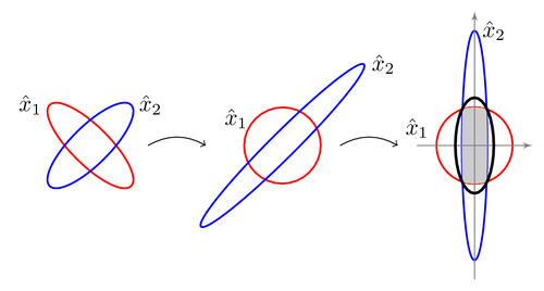
Graphical interpretation of an algorithm for fusing two estimates in a safe way. The ellipses are the covariances of the estimates.
Note how the red ellipse is transformed to a unit circle using the xscale and yscale options. As a result the blue ellipse is squeezed.
Edit and compile if you like:
\documentclass{article}
\usepackage{tikz}
\usetikzlibrary{arrows}


\begin{document}
\pagestyle{empty}

\def\Pi{(0,0) ellipse (1.5 and 0.5)} % Covariance of xhat_1
\def\Pii{(0,0) ellipse (.5 and 1.5)} % Covariance of xhat_2
\tikzstyle{P_1} = [draw,red,thick]
\tikzstyle{P_2} = [draw,blue,thick]

\begin{tikzpicture}[scale=0.6,>=latex']
    \begin{scope}[rotate=-45]
        \path[P_1] \Pi;
        \path[P_2] \Pii;
        \path (-1.5,0) node[left] {$\hat{x}_1$}
            (0,1.5) node [right] {$\hat{x}_2$};
    \end{scope}
    % Note that the order of the transformation options is important.
    % The last transformation is applied first.
    \begin{scope}[xshift=5cm,rotate=-45, xscale=0.66, yscale=2]
        \path[P_1] \Pi;
        \path[P_2] \Pii;
        \path (-1.5,0) node[left] {$\hat{x}_1$}
            (0,1.5) node [right] {$\hat{x}_2$};
    \end{scope}
    \begin{scope}[xshift=10cm,rotate=0,xscale=0.66, yscale=2]
        \path[P_1] \Pi;
        \path[P_2] \Pii;
        \path (-1.5,0) node[above left] {$\hat{x}_1$}
              (0,1.5) node [right] {$\hat{x}_2$};
        % Fill intersection between P_1 and P_2. Use P_1 as clipping path
        \clip \Pi;
        \fill[fill=black!20] \Pii;
    \end{scope}
    \begin{scope}[xshift=10cm]
        \draw[thin,->,black!50] (-1.5,0) -- (1.5,0);
        \draw[thin,->,black!50] (0,-3.5) -- (0,3.5);
        \draw[very thick] (0,0) ellipse (0.5 and 1.25);
    \end{scope}
    \draw[-to] (1.5,0) to[bend left] (3.0,0);
    \draw[-to] (6.5,0) to[bend left] (8.0,0);
\end{tikzpicture}


\end{document}
Click to download: safe-fusion.tex • safe-fusion.pdf
Open in Overleaf: safe-fusion.tex