


With PGF/TikZ version 1.09 and later, it is possible to draw paths between nodes across different pictures. This is a useful feature for presentations with the Beamer package. In this example I've combined the new PGF/TikZ's overlay feature with Beamer overlays. Download the PDF version to see the result.
Note. This only works with PDFTeX, and you have to run PDFTeX twice.
Author: Kjell Magne Fauske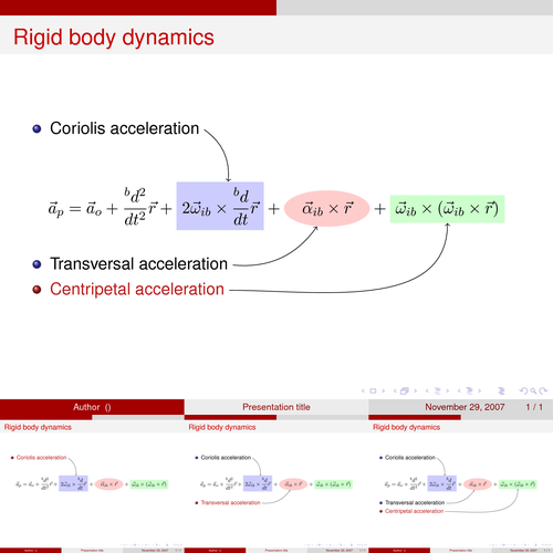
Edit and compile if you like:
\documentclass{beamer} %
\usetheme{CambridgeUS}
\usepackage[latin1]{inputenc}
\usefonttheme{professionalfonts}
\usepackage{times}
\usepackage{tikz}
\usepackage{amsmath}
\usetikzlibrary{arrows,shapes}

\author{Author}
\title{Presentation title}

\begin{document}


% For every picture that defines or uses external nodes, you'll have to
% apply the 'remember picture' style. To avoid some typing, we'll apply
% the style to all pictures.
\tikzstyle{every picture}+=[remember picture]

% By default all math in TikZ nodes are set in inline mode. Change this to
% displaystyle so that we don't get small fractions.
\everymath{\displaystyle}

\begin{frame}
\frametitle{Rigid body dynamics}

\tikzstyle{na} = [baseline=-.5ex]

\begin{itemize}[<+-| alert@+>]
    \item Coriolis acceleration
        \tikz[na] \node[coordinate] (n1) {};
\end{itemize}

% Below we mix an ordinary equation with TikZ nodes. Note that we have to
% adjust the baseline of the nodes to get proper alignment with the rest of
% the equation.
\begin{equation*}
\vec{a}_p = \vec{a}_o+\frac{{}^bd^2}{dt^2}\vec{r} +
        \tikz[baseline]{
            \node[fill=blue!20,anchor=base] (t1)
            {$ 2\vec{\omega}_{ib}\times\frac{{}^bd}{dt}\vec{r}$};
        } +
        \tikz[baseline]{
            \node[fill=red!20, ellipse,anchor=base] (t2)
            {$\vec{\alpha}_{ib}\times\vec{r}$};
        } +
        \tikz[baseline]{
            \node[fill=green!20,anchor=base] (t3)
            {$\vec{\omega}_{ib}\times(\vec{\omega}_{ib}\times\vec{r})$};
        }
\end{equation*}

\begin{itemize}[<+-| alert@+>]
    \item Transversal acceleration
        \tikz[na]\node [coordinate] (n2) {};
    \item Centripetal acceleration
        \tikz[na]\node [coordinate] (n3) {};
\end{itemize}

% Now it's time to draw some edges between the global nodes. Note that we
% have to apply the 'overlay' style.
\begin{tikzpicture}[overlay]
        \path[->]<1-> (n1) edge [bend left] (t1);
        \path[->]<2-> (n2) edge [bend right] (t2);
        \path[->]<3-> (n3) edge [out=0, in=-90] (t3);
\end{tikzpicture}
\end{frame}
\end{document}
Click to download: beamer-arrows.tex • beamer-arrows.pdf
Open in Overleaf: beamer-arrows.tex