


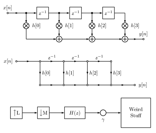
This library is an extension of the example of Karlheinz Ochs [1] and provides basic building blocks for block diagrams and signal flow graphs. The provided example illustrates a finite impulse response (FIR) filter as block diagram and signal flow graph.
[1] /signal-flow-building-blocks/
Edit and compile if you like:
% Library for block diagrams and signal flow graphs
% Author: Matthias Hotz
\documentclass{article}
\usepackage{tikz}
\usepackage[active,tightpage]{preview}
\PreviewEnvironment{tikzpicture}
\setlength{\PreviewBorder}{10pt}%
\usetikzlibrary{dsp,chains}

\DeclareMathAlphabet{\mathpzc}{OT1}{pzc}{m}{it}
\newcommand{\z}{\mathpzc{z}}

\begin{document}
% FIR filter as block diagram
\begin{tikzpicture}

	% Place nodes using a matrix
	\matrix (m1) [row sep=2.5mm, column sep=5mm]
	{
		%--------------------------------------------------------------------
		\node[dspnodeopen,dsp/label=above] (m00) {$x[n]$};    &
		\node[coordinate]                  (m01) {};          &
		\node[dspnodefull]                 (m02) {};          &
		\node[dspsquare]                   (m03) {$\z^{-1}$}; &
		\node[dspnodefull]                 (m04) {};          &
		\node[dspsquare]                   (m05) {$\z^{-1}$}; &
		\node[dspnodefull]                 (m06) {};          &
		\node[dspsquare]                   (m07) {$\z^{-1}$}; &
		\node[coordinate]                  (m08) {};          &
		\node[coordinate]                  (m09) {};          &
		\node[coordinate]                  (m0X) {};          \\
		%--------------------------------------------------------------------
		\node[coordinate]                  (m10) {};          &
		\node[coordinate]                  (m11) {};          &
		\node[dspmixer, dsp/label=right]   (m12) {$h[0]$};    &
		\node[coordinate]                  (m13) {};          &
		\node[dspmixer, dsp/label=right]   (m14) {$h[1]$};    &
		\node[coordinate]                  (m15) {};          &
		\node[dspmixer, dsp/label=right]   (m16) {$h[2]$};    &
		\node[coordinate]                  (m17) {};          &
		\node[dspmixer, dsp/label=right]   (m18) {$h[3]$};    &
		\node[coordinate]                  (m19) {};          &
		\node[coordinate]                  (m1X) {};          \\
		%--------------------------------------------------------------------
		\\
		%--------------------------------------------------------------------
		\node[coordinate]                  (m20) {};          &
		\node[coordinate]                  (m21) {};          &
		\node[coordinate]                  (m22) {};          &
		\node[coordinate]                  (m23) {};          &
		\node[dspadder]                    (m24) {};          &
		\node[coordinate]                  (m25) {};          &
		\node[dspadder]                    (m26) {};          &
		\node[coordinate]                  (m27) {};          &
		\node[dspadder]                    (m28) {};          &
		\node[coordinate]                  (m29) {};          &
		\node[dspnodeopen,dsp/label=above] (m2X) {$y[n]$};    \\
		%--------------------------------------------------------------------
	};

	% Draw connections

	\begin{scope}[start chain]
		\chainin (m00);
		\chainin (m02) [join=by dspflow];
		\chainin (m12) [join=by dspconn];
		\chainin (m22) [join=by dspline];
	\end{scope}

	\foreach \i [evaluate = \i as \j using int(\i+1),
	             evaluate = \i as \k using int(\i+2),] in {2,4,6}
	{
		\begin{scope}[start chain]
			\chainin (m0\i);
			\chainin (m0\j) [join=by dspconn];
			\chainin (m0\k) [join=by dspline];
			\chainin (m1\k) [join=by dspconn];
			\chainin (m2\k) [join=by dspconn];
		\end{scope}
		\draw[dspconn] (m2\i) -- (m2\k);
	}

	\draw[dspflow] (m28) -- (m2X);


	% Place nodes using another matrix for another picture
	\matrix (m2) [row sep=15mm, column sep=15mm, below=of m1]
	{
		%--------------------------------------------------------------------
		\node[dspnodeopen,dsp/label=left]  (m00) {$x[n]$};  &
		\node[dspnodeopen]                 (m01) {};        &
		\node[dspnodeopen]                 (m02) {};        &
		\node[dspnodeopen]                 (m03) {};        &
		\node[dspnodeopen]                 (m04) {};        &
		\node[coordinate]                  (m05) {};        \\
		%--------------------------------------------------------------------
		\node[coordinate]                  (m10) {};        &
		\node[dspnodeopen]                 (m11) {};        &
		\node[dspnodeopen]                 (m12) {};        &
		\node[dspnodeopen]                 (m13) {};        &
		\node[dspnodeopen]                 (m14) {};        &
		\node[dspnodeopen,dsp/label=right] (m15) {$y[n]$};  \\
		%--------------------------------------------------------------------
	};

	% Draw connections

	\draw[dspflow] (m00) -- (m01);

	\foreach \i [evaluate = \i as \j using int(\i+1)] in {1,2,3}
		\draw[dspflow] (m0\i) -- node[midway,above] {$\z^{-1}$} (m0\j);

	\foreach \i [evaluate = \i as \j using int(\i-1)] in {1,2,...,4}
		\draw[dspflow] (m0\i) -- node[midway,right] {$h[\j]$} (m1\i);

	\foreach \i [evaluate = \i as \j using int(\i+1)] in {1,2,...,4}
		\draw[dspflow] (m1\i) -- (m1\j);

	% Other elements
	\node[dspsquare, below=of m10, below=10ex]       (c0) {\upsamplertext{L}};
	\node[dspsquare,right= of c0]                    (c1) {\downsamplertext{M}};
	\node[dspfilter,right=of c1]                     (c2) {$H(\z)$};
	\node[dspmultiplier,right=of c2,dsp/label=below] (c3) {$\gamma$};
	\node[dspfilter,right=of c3,minimum size=2cm,text height=2em]
	                                                 (c4) {Weird\\ Stuff};
	\foreach \i [evaluate = \i as \j using int(\i+1)] in {0,1,...,3}
		\draw[dspconn] (c\i) -- (c\j);
\end{tikzpicture}

\end{document}
Click to download: fir-filter.tex • fir-filter.pdf
Open in Overleaf: fir-filter.tex