Finite impulse response filter

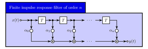
Illustration of a finite impulse response filter of order n. The drawing is made using the signalflow library made by Karlheinz Ochs. The signalflow library is a specialized library for drawing signal flow diagrams, commonly found in the digital signal processing and control theory literature

The library defines several custom node shapes like the multiplier, delay, terminal, and adder shapes. Of special interest is the multiplier shape that places the node label outside the circle.

The library also defines the tikzgrid environment, which is a convenient way of arranging nodes in grids using the familiar array syntax. Furthermore the library defines several domain specific styles for elements like for instance real valued and complex valued signals.

Files:

• Download the version of the signalflow library used in this example: signalflowlibrary.zip

Edit and compile if you like:

% Example for an interconnection of signal flow diagrams.
%
% Author: Dr. Karlheinz Ochs, Ruhr-University of Bochum, Germany
% Version: 0.1
% Date: 2007/01/05
\documentclass{article}
\usepackage{signalflowdiagram}

\usepackage[active,tightpage]{preview}
\PreviewEnvironment{signalflow}
\setlength\PreviewBorder{5pt}%


\pagestyle{empty}

\begin{document}


% An FIR filter
\begin{signalflow}[node distance=9mm]{Finite impulse response filter of order $n$}%
   % The \tikzgrid environment creates a fixed sized grid, where each
   % node in the grid is placed using the familiar array syntax.
   % The grid size is set using the node distance option.
   % Tip: Use the xscale and yscale options to get different spacing in the
   %      x and y directions.
   \tikzgrid{
      % building blocks
      \node[input]      (in)  {$x(t)$}     &
      \node[node]       (n0)  {}           &
      \node[delay]      (d1)  {$T$}        &
      \node[node]       (n1)  {}           &
      \node[delay]      (d2)  {$T$}        &
      \node[node]       (n2)  {}           &
      \node[coordinate] (c1)  {}           &
      \node[coordinate] (c3)  {}           &
      \node[delay]      (dn)  {$T$}        &
      \\ &
      \node[multiplier] (m0)  {$\alpha_0$} & &
      \node[multiplier] (m1)  {$\alpha_1$} & &
      \node[multiplier] (m2)  {$\alpha_2$} & & & &
      \node[multiplier] (mn)  {$\alpha_n$}
      \\ & & &
      \node[adder]      (a1)  {}           & &
      \node[adder]      (a2)  {}           &
      \node[coordinate] (c2)  {}           &
      \node[coordinate] (c4)  {}           & &
      \node[adder]      (an)  {}           &
      \node[output]     (out) {$y(t)$}
   }
   % signal paths
   % r is short hand notation for a real signal.
   % Use c to get a complex style signal
   \path[r>] (in) -- (n0);
   \path[r>] (n0) -- (d1);
   \path[r>] (d1) -- (n1);
   \path[r>] (n1) -- (d2);
   \path[r>] (d2) -- (n2);
   \path[r>] (n2) -- (c1); % continuation
   \path[r.] (c1) -- (c3); % continuation
   \path[r>] (c3) -- (dn); % continuation
   \path[r>] (n0) -- (m0);
   \path[r>] (n1) -- (m1);
   \path[r>] (n2) -- (m2);
   \path[r>] (dn) -| (mn);
   \path[r>] (m0) |- (a1);
   \path[r>] (m1) -- (a1);
   \path[r>] (m2) -- (a2);
   \path[r>] (mn) -- (an);
   \path[r>] (a1) -- (a2);
   \path[r>] (a2) -- (c2); % continuation
   \path[r.] (c2) -- (c4); % continuation
   \path[r>] (c4) -- (an); % continuation
   \path[r>] (an) -- (out);
\end{signalflow}


\end{document}